Parallel Computing Intro
Introduction
Many compute tasks benefit from running in parallel, that is: executing multiple parts of the task simultaneously. This can be done on a single machine (your laptop or workflow head node) or on a cluster or grid of machines.
Before delving into parallel and grid computing though, let’s establish some basics of computing. We will discuss:
computing => parallel computing => grid computing
Computing basics
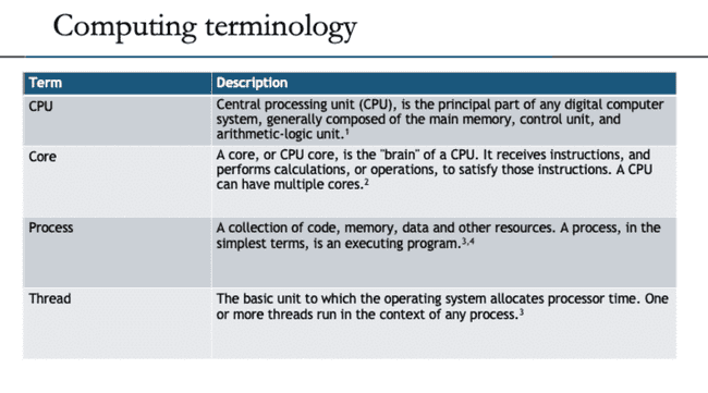
The goal of this section is to provide a high-level view of how a computer does work. It is helpful to understand these basic concepts before thinking about how a computer does work in parallel.
CPU core execution
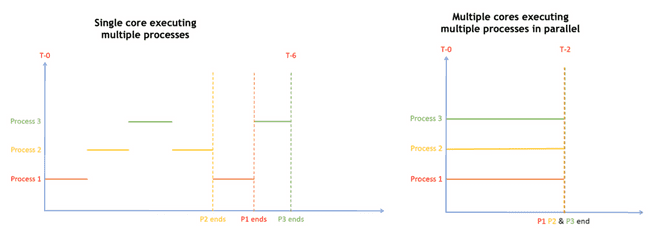
A single core only executes a single process (actually a single thread) at any given time. However, the OS scheduler is constantly swapping which processes are actually executing based on when the current process is waiting on something like user input or reading from disk or network.
Parallel processing
Some compute tasks benefit from being able to run multiple parts of the task in parallel, that is: simultaneously. This requires multiple cores, because a single CPU core only executes one process at a time (see caveat on hyperthreading, below).
A little later, we will discuss different types of tasks and which are generally better suited for parallelization. But first, we’ll lay out some basic concepts.
Processes and threads
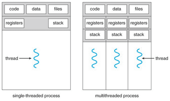
Any process has one or more threads. Threads are lighter-weight because they share the memory space of the process that spawned them.
Some languages like Go, Java, and C use threading to efficiently parallelize work, as opposed to spawning entirely new processes.
Single-threaded processes
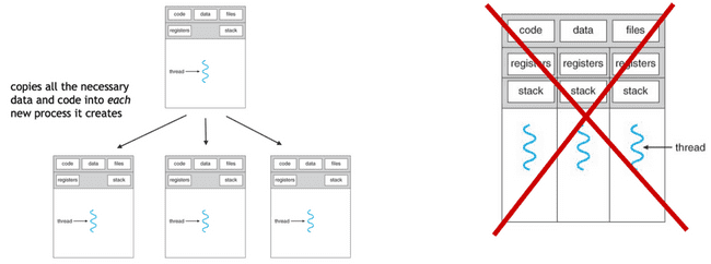
R and NONMEM are single-threaded. This means that each new parallel process you launch is, in fact, a process which has its own memory space, etc.
Primarily because each new process has to copy all of the data, etc., there is a fair amount of overhead for each process that is created. Accessing, copying, and moving data is extremely slow, as compared to processing data. This means that there is overhead to starting new processes in this way, and this overhead sometimes overwhelms the gains of doing the actual processing in parallel.
Note: any time you are parallelizing in R or NONMEM, this is what is happening. (The only exception to this is using "forking", which has its own drawbacks and is discussed below.)
Caveat on hyperthreading
Hyperthreading allows a single CPU core to run two (or potentially more) threads at once. This is used by default on AWS, so 8 “vCPU’s” actually means 4 physical CPU cores that can each run two threads. There is some nuance to this that is beyond the scope of this article. For now, know that conceptually it is the same as twice as many cores, but in reality it is not twice as fast, typically more like 1.5x as fast.
Consider your process
Before deciding how many (if any) processes you want to parallelize to, you need to think about how much time will be spent moving data around vs. actually doing computational work.
Example 1: a poor candidate for parallel
Consider the following process that has roughly 2 minutes of data I/O (input/output, i.e. moving data around from disk or between processes) and roughly 10 minutes of actual computation (doing math, etc.).
It would be nice if parallelizing this over 4 workers would make it 4x faster. Indeed, even if the I/O was a sunk cost up front, this wouldn't be too bad.
However, what actually happens is this:
The parent process needs to spend some time spinning off each of the child processes to do work, and then it needs to pass the necessary data to each of them. The important point here is that, even though you are distributing the core computational work, the parent process can still only do one thing at a time which means any communication with child processes is done sequentially.
Now imagine that you naively want to speed this up more, so you decide to distribute this same job over 8 workers. Now we get this:
The job now ends up taking longer because the parent process is spending so much time spawning children and sending them data that it outstrips the gains you have gotten from each child process doing its computation in less time. This is a big pitfall in parallel processing: in these situations distributing to more cores can sometimes slow down your total run time.
Example 2: A better candidate for parallel
Now consider a different process that still has roughly 2 minutes of I/O time, but has roughly an hour of computation. Imagine this is a more complex model, but using the same input data.
Now we get a significant speed up. Because the I/O time was relatively small compared to the compute time, the gains from doling out the computation to workers far outweigh the work done by the parent process to spawn those workers and send them the data.
Takeaway: don't over-parallelize
Over-parallelizing (i.e. using more workers than your process merits) will slow down your code, sometimes significantly. Start small (e.g. 4 workers) and work your way up when you’re sure your process needs the extra compute resources.
It is often a good idea, when you are running something that you think will benefit from heavy parallelization, to run some testing iterations first, before kicking off a potentially long-running job. See the "Testing different numbers of threads" section in this Running NONMEM in Parallel: bbr Tips and Tricks vignette.
Nested parallelism
Nested parallelism is when you have jobs executing in parallel and those jobs attempt to launch more jobs to execute in parallel. As you can imagine, this should be handled with care.
Unintentional nested parallelism
There are times when you intend to do this, but first we will talk about some scenarios when it happens unintentionally because something you’re using is parallelizing under the hood. Two common examples:
- Processes doing heavy linear algebra (BLAS and LAPACK)
- Using
data.table::fread()
There's a good summary of this issue in the “Hidden Parallelism” section of Roger Peng R Programming for Data Science.
Intentional nested parallelism
Sometimes you will have a situation where you have two (or more) levels of computation that could be parallelized. Examples include:
- Running multiple NONMEM models at once and wanting each model to run on multiple cores.
- Running a Bayesian model with four chains; wanting to run the chains in parallel and also parallelize computation within each chain.
- Splitting a data set into subgroups and running multiple simulations on each subgroup.
These tasks can certainly be accomplished by running them on a single very large machine that has enough cores for all the workers that will be spawned.
However, in many cases, it is cheaper—both in run time and AWS costs—to... take it to The Grid!
Sidebar: bootstraps
Note that if you’re running a lot of models at once (e.g. a bootstrap) then you can easily run into the same pitfalls as BLAS or data.table. In these cases, it’s usually best to run each model on a single core and parallelize across models instead, for example with bbr::submit_models().
The grid
Parallel computing is great, and parallelizing on a single machine works well for many tasks. But for others, especially large tasks and tasks involving nested parallelism, using a “grid” or “cluster” of multiple machines has many advantages. For example:
- Auto-scaling: the grid will launch new workers when they have tasks to run, and then tear them down when the tasks are finished. This saves on compute costs because we don't have to pay for idle resources.
- Job queueing: you can launch jobs without worrying about currently available resources because the grid will keep them in a queue until it has the resources to run them.
- Spot instances: Metworx is configured to use AWS “spot instances” for worker nodes, which makes them much cheaper.
Each Metworx workflow is your own personal grid.
The structure of the grid
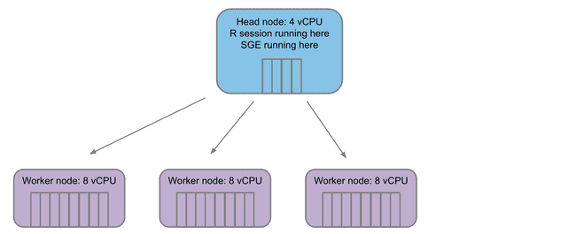
Any grid will have a single head node. This is the machine that is coordinating which jobs, if any, are sent off to compute nodes. The head node is also where things like your Rstudio session are running.
When jobs are submitted to the grid, the head node launches some number of worker nodes (based on the workload submitted) and fills a queue for the workers to pull jobs from.
Configuring your grid on Metworx
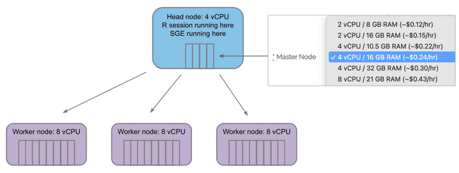
The Master Node menu selects how many vCPU "cores" are on the master/head node. Remember, you will only ever have one master/head node.
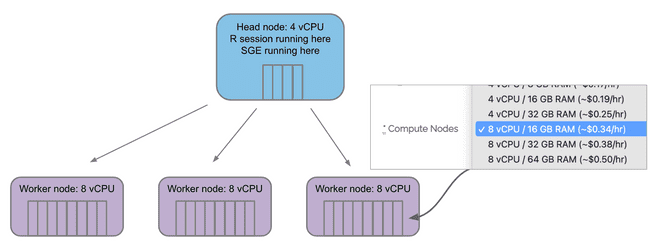
The Compute Nodes menu selects how many vCPU "cores" are on each compute/worker node.
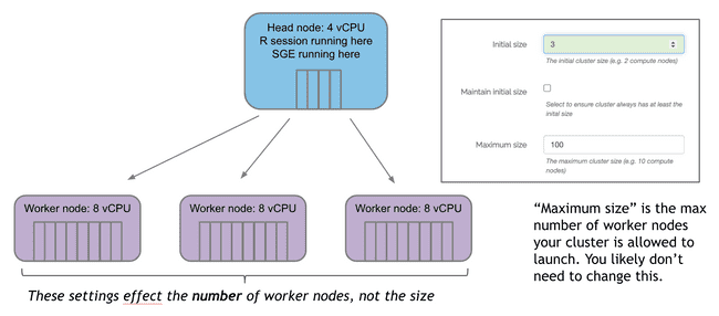
Initial size specifies how many worker nodes will be created at launch.
If no jobs are submitted, these will countdown to terminating unless “Maintain initial size” is checked. Note: this box should be used with caution. Auto-scaling is a good thing. You don’t want workers sitting around doing nothing for long periods of time because they cost money. Unless you have a good reason that you can't wait for workers to scale up (typically 3-5 minutes from when jobs are submitted) it is much more cost effective to leave this box unchecked and let the auto-scaling handle the number of worker nodes.
Grid terminology
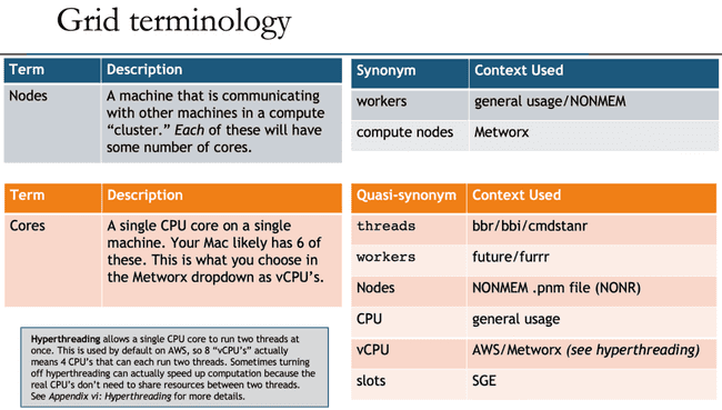
Unfortunately, as with many technology disciplines, grid computing uses a wide range of terminology to describe essentially the same concepts. For one thing, the terms "grid" and "cluster" are often used interchangeably (although there are slight technical differences). Additionally, the head node is often called the "master" node, though that term is getting phased out for inclusivity reasons (similar to how Github has renamed to the main branch). Likewise, the worker nodes are sometimes called "compute" nodes.
Beyond that, the concepts of "nodes" (physical machines) and "cores" (CPU cores on those machines) have many quasi-synonyms that muddy the waters even further.
To further confuse things, you may notice that NONMEM (and most people in general) refer to nodes when they say "workers", but the workers argument in functions from the future and furrr packages actually refers to the number of jobs to spawn, which is likely equal to your number of cores. And, even more confusingly, the NONMEM .pnm file refers to nodes at WORKERS and cores as NODES. (There is a historical reason for this, but in 2021 it definitely feels deserving of a facepalm emoji.)
All that is to say: don't be discouraged if you are confused by terminology, and please refer back to the above table when this confusion inevitably happens.
Submitting jobs to the grid
The diagrams below illustrate what is happening when you submit jobs to be run on the worker nodes of the grid. In this case, we are using bbr to submit NONMEM jobs from R.As a side note, if you are using bbr to submit NONMEM jobs on the grid, consider reading this Running NONMEM in Parallel: bbr Tips and Tricks vignette for more details and best practices.
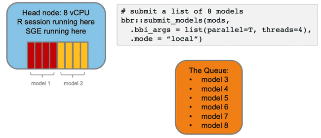
Imagine you want to submit some NONMEM models to run on your head node via bbr. You specify that they should run in parallel and each model should use 4 cores (threads).
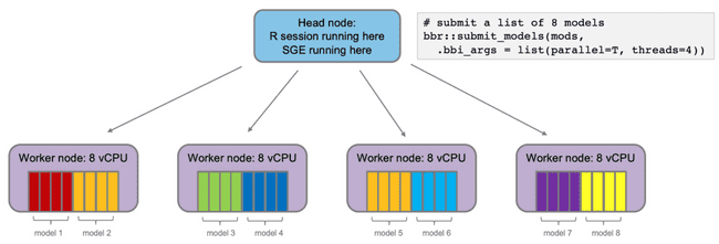
Now, imagine you want to submit some NONMEM models to run on the grid via bbr. Again, you want to run in parallel and each model should use 4 cores (threads).
The head node will submit the jobs to the SGE queue, which will distribute them to the worker nodes. With 4 worker nodes, all models will run simultaneously. This is good.
Monitoring parallelization
It can sometimes be disconcerting to launch some large jobs in parallel and then think "I wonder if they're actually working..." Luckily, there are several ways to monitor these jobs.
Monitoring "locally" on the head node
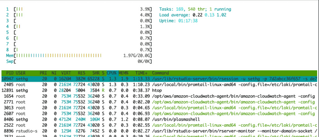
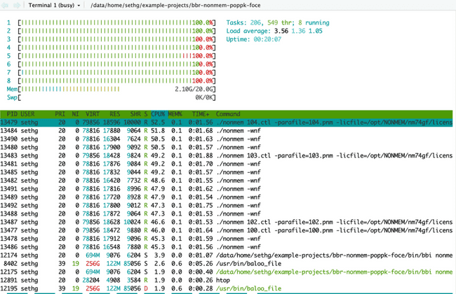
When running jobs in parallel on your head node, probably the easiest way to monitor if they are running (and using the expected number of cores) is to use the Linux utility htop. In your terminal (not your R console) simply type htop. This brings up the following visual:
The horizontal bar graph at the top tells you (among other things) about the cores on your machine and how much each is being used. There is a bar for each core (each vCPU actually) and they will be lit up green to show percent utilization. The table underneath shows all currently running processes. (You might be amazed to see how many there are at any given time, and how little CPU most of them use...) This is essentially the same thing you see in top (another common Linux utility for monitoring processes).
Below is htop after submitting eight NONMEM models, each using four cores (this is the first example in the "Submitting jobs to the grid" section above). Notice all cores are lit up green because we have submitted (more than) enough work to use all available CPU resources.
You can quit at any time with ctrl+C or F10 and get back to your terminal.
Monitoring on the grid
If you are submitting jobs to be run on the grid, you won't see them in htop because htop only monitors the head node.
However, there are several other tools for monitoring work being done on the grid. The following examples are showing monitoring from submitting eight NONMEM models to run on the grid, using four cores for each model. This is the second example from the "Submitting jobs to the grid" section above.
Grafana
Starting with the 21.08 release, Metworx is configured to display usage information in a Grafana dashboard. You can access this simply by adding grafana to the end of your workflow URL, like https://i-0972bb95cd8cb78ec.metworx.com/grafana. There is a helpful "Getting Started With Grafana" article here.
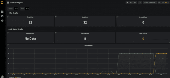
The top of the dashboard shows some high-level stats about utilization across the entire grid.
Here we can see that we have 32 available "slots" (a.k.a. cores, refer to "Grid terminology" section above). This is because we have four worker nodes up, each of which has eight cores. Furthermore, you can see that they are all in use, because we have submitted eight models to run, and asked for each to use four cores (8 * 4 = 32).
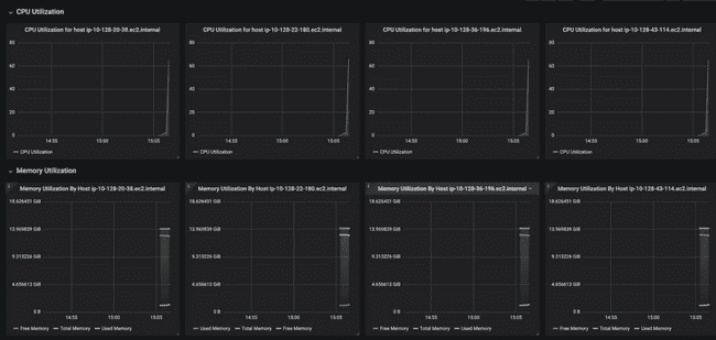
Below that, the dashboard shows CPU and memory usage for each worker node. Notice how each of them has a small peak to the right-hand side, showing that they have each just started working on something (the job we submitted).
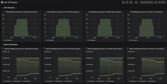
And this is ten minutes later, when all the jobs have finished. You can see that CPU utilization on each node went to 100% for roughly seven minutes while the models were running. You can also see the "used memory" line (annoyingly, different colors for each node) creep up as the models run, though never coming close to using all the memory.
As a sidenote, if you had looked at htop during this period, you would not see any activity, because all processing was done on the worker nodes and htop, as previously stated, only show activity on the head node.
qstat
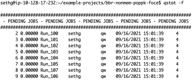
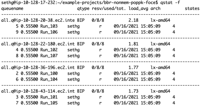
You can also use the qstat command (also used in the terminal, not the R console) to show you the jobs currently queued or running on the grid. (The -f flag shows a more informative output.)
Here is qstat -f right after the jobs were submitted, before any worker nodes have come up to process them:
And here is qstat -f showing all eight jobs being processed simultaneously, on four 8-core worker nodes (as shown in the diagram at the end of the "Submitting jobs to the grid" section).
Conclusion
Hopefully this was a helpful introduction to the concepts of parallel and grid computing. For more details, on this content, please reference the "Intro to Grid Computing" JET slide deck that this article is based on. Also, please reference the other KB pages linked in the introduction for more detail on specific applications of this content.
